I’ve spent the past six or so weeks working on a system that can generate realistic, labeled computer vision datasets from virtual scenes. This project was inspired by my time spent working at PFF earlier in the summer, a lot of which centered around creating a simulated testing environment in Gazebo. Access to Gazebo reduced our testing dependencies on the limited amount of prototype robots we had around, and I feel that it was generally helpful. However, I also found that the simulation did not help very much for testing the computer vision aspect of our product, which still relied heavily on manually gathered data. I felt that simulation offered a great avenue for automated generation of this type of data, and had the added benefit of easy access to ground truth values, which were almost never available when collecting data from physical sensors.
So, after finishing my internship and taking a little vacation, I decided that I would explore this sort of technology on my own. I wasn’t necessarily after results - I just wanted to learn about how a system like this might fit into a computer vision training pipeline. I had never done any real work with neural networks before, so this was a good excuse to learn about those, too. With my graduation and first full-time job (hopefully in CV/robotics) looming on the horizon, I figured a little extra domain knowledge here could go a long way.
Project Goals
As this was primarily an exploratory project, I started with some fairly broad goals. First and foremost, I wanted render realistic data for supervised training of some sort of computer vision model. Secondly, I wanted to show that my method could generate data of comparable quality to stuff produced in the “real world”. I started in the last week of July and gave myself until the beginning of the semester to get a finished product.
Selecting a Task and Dataset
To start this project, I needed to pick a task to train my model for, as well as a respected dataset to use for training of a baseline. Semantic image segmentation (labeling each pixel of an image based on a predefined set of classes) seemed to be a good fit here, as I had a hunch that generating synthetic data for this sort of task would be relatively straightforward. Other than the actual render, I would only need to output an identically sized, single channel image with each pixel representing a label. I figured that this could be done by an existing rendering engine without many modifications, and some searching of the Blender documentation confirmed this.
Choosing the dataset was a little trickier. Initially, I wanted to do something with outdoor scenes from a car’s perspective. I even found a good dataset for this sort of project. However, the task of finding, placing, and animating models of pedestrians, trees, cars, etc. in a dynamic urban environment seemed a little too difficult given my time constraints. I feared that taking on this sort of thing would quickly devolve into a computer animation project, which would’ve been cool, but wasn’t what I was going for. Still, it would be awesome to make an entire city with something like this and generate hours of perfectly labeled driving data. The pinnacle of this sort of platform would probably look a lot like the OpenAI GTA V integration that has since mysteriously disappeared.
Alas, to keep things manageable, I settled on finding semantic segmentation datasets of static, interior scenes. ADE20K was the first one I stumbled upon, but I found that it had too wide of a variety of scenes, and went far too granular with its labeling by separating out individual body parts and the like. I then discovered that ADE20K is partially built on the MIT SUN dataset, which is in turn partially built on the NYU Depth Dataset V2. Compared to the other datasets, the NYU is very focused in terms of the types of depicted objects. Most of the images feature interior scenes in houses and offices with no humans present, and objects labels are simple and often fairly broad (chair, wall, table, and so on). Because I knew that I could easily find free, premade assets for these kinds of scenes online, I decided that the NYU dataset would be a perfect fit for a baseline dataset.
Training and Assessing the Baseline Model
With dataset and task in hand, I set out to train a baseline segmentation model to measure the “realness” of my synthetic dataset against. To ensure that the potential performance of my model would be consistent with modern best practices, I opted to use this Caffe implementation of the SegNet architecture. It had decent documentation, and someone had even trained it on the SUN dataset before, so I had no doubt that it could perform decently on the NYU dataset.
Training the model was easily the hardest part of the project. My lack of experience with neural nets meant that I had to lean heavily on trial and error to get things working. Even when things started working, I often had no intuition if my results were “good” or not. What is a reasonable learning rate? What sort of accuracy should I be looking for after 10 epochs? After 100 epochs? How long should I let the thing train for before shutting it down? These sorts of little questions were often major roadblocks, as every little tweak would require restarting hours of training in order to even see any effects. It was maddening to know that most of these questions could probably have been answered by a domain expert in less than a minute, saving me literal days of effort. I usually enjoy learning this sort of stuff on my own, at my own pace, but this whole process really had me wishing for easy access to a mentor or adviser.
Speaking of wasted time, man did I ever underestimate how resource-intensive this stuff is. I went into this project thinking that it would be a good way to get some use out of my newly assembled computer’s GPU. I spent a day trying to get the provided GPU-enabled docker image working on my machine, only to find that I don’t have enough VRAM to even run training at the smallest batch size with downsampled images. After this, I ran the horrendously slow CPU-based training for about a day before deciding it wasn’t worth it. With my system maxed out, I would’ve needed to train for something on the order of weeks in order to process the number of epochs suggested by the tutorial. Finally, I decided to use my $300 of account credit on Google Cloud Platform to rent an instance with a GPU. I never thought I would be pleased to see a program taking 48 hours to run, but in this case, it was a huge relief.
Initially, I split the dataset of ~1400 images 80/20, using the first 80% of images for training and the rest for testing. I also wrote some scripts to extract all images and labels into formats that SegNet liked, removing all but the 30 most prevalent labels (down from around 900). At this point, the least common label was only present in around 12% of the training set, which I thought was a decent cutoff.
Then came the tweaking. It was always little things, like the fact that the NYU dataset uses 0 as its “unlabeled” label whereas SegNet requires the unlabeled pixel value to be greater than all others. Or realizing that objects that are neither unlabeled nor one of the 30 most common should be considered unlabeled, not simply lumped into a giant “other” label (in hindsight, this was a dumb mistake). None of these changes took more than a couple minutes to actually implement, but the fact that they were followed by batch processing of 1400 images + hours of training was really a killer. Other small changes included reducing the number of classes to 16 (to improve average accuracy), and shuffling the data before dividing into testing and training sets (as images of the same type of location were often clumped together).
Finally, I managed to get a result that I was happy with. I stopped training at 240 epochs (40,000 iterations with batch size 7), though it looked like the model could’ve continued to improve with some more training. This resulted in an average class accuracy of 94.51% and a global accuracy of 56.11%. I was a little confused by the fact that average class accuracy is higher than global accuracy - something that didn’t happen in any of the results published in the SegNet paper. This led me to believe that I had written the accuracy grading scripts wrong, but after triple checking, I’m pretty sure that I’ve written them correctly. My theory is that, because accuracy weights true negatives and true positives equally, less common labels will tend to appear highly accurate even if there are never any predicted positives. For example, the least common label, “sink”, had 99.56% class accuracy, but it could be the case that the model simply learned to never predict sink, causing the massive amount of true negatives to mask the minimal amount of false ones. A better breakdown of precision/recall would probably be good here.
Generating Synthetic Data
After getting intimately familiar with the model input format and the types of images in the dataset, I started work on generating the synthetic images. Because I had a little previous experience with it, I planned on doing all of the rendering with Blender and the Cycles rendering engine. Initially, my plan was to find free models of furniture online, then arrange them into scenes. However, after a little poking around, I realized that I could get entire interior scenes for free. This saved me from spending a lot of time fixing compatibility issues with imported models, lighting scenes, and doing other little things. I selected about six scenes of various rooms that one might find in a normal-looking house.
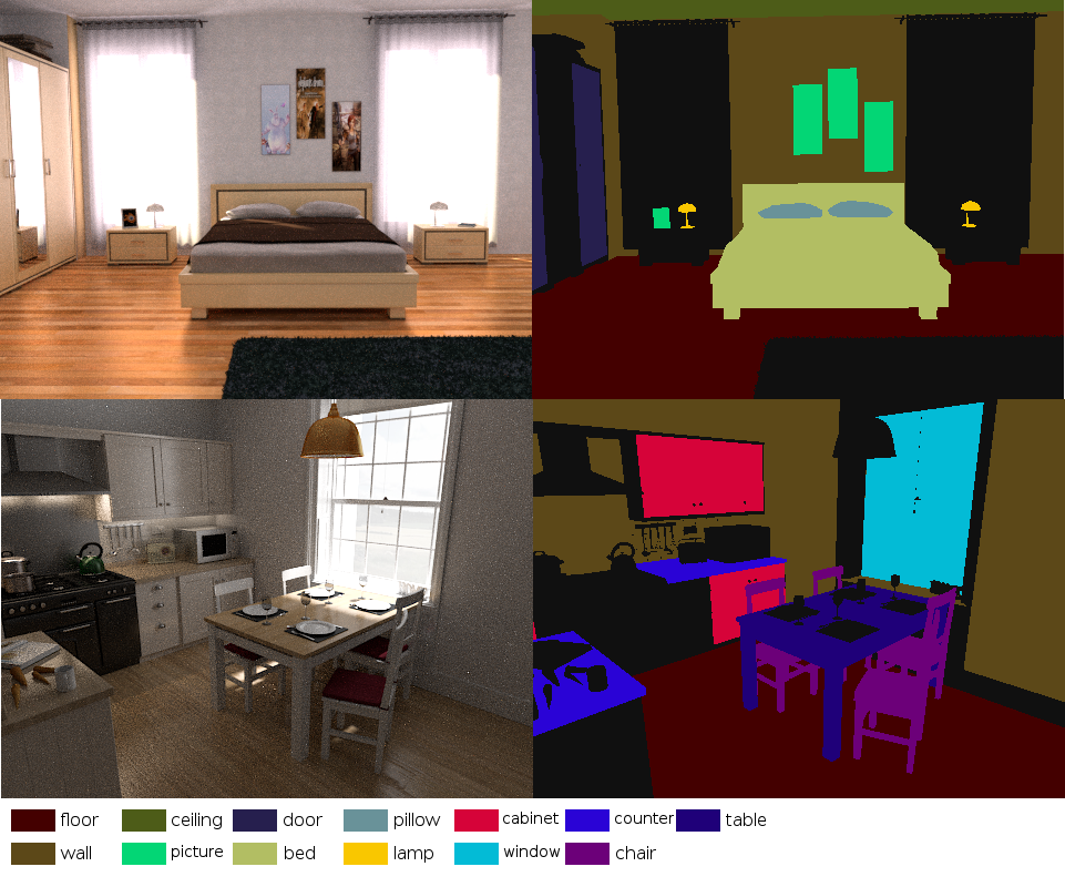
Because the scenes were pre-lit and everything, rendering was easy. For each scene, I would animate the camera to jump between three or four angles, squeezing as many varied images as possible out of each scene. To output the label images I needed, I made use of Blender’s built-in render passes - specifically, the object index pass. This pass lets you assign each object a “pass index”, then outputs an image where each object in the scene is masked by its pass index value. I wrote a small Blender add-on that let me assign selected objects the correct pass index for their label, then went through all scenes assigning the labels to the relevant objects. Sometimes, I would need to separate some pieces of meshes out into separate objects (like separating closet doors from the rest of the closet mesh) so that I could accurately label the different parts. Once this was done, I would run another Blender script to set the correct image dimensions, output locations, and do other little housekeeping things. Because Blender’s scale for pixel values is between 0 and 1.0, but the object index pass outputs from 0 to NUM_LABELS, the script also adds a compositing node to divide all the object index values by 255. This way, once the images are saved, each label pixel has the proper value between 0 and NUM_LABELS. Once a scene has been processed like this, all that’s left to do is render the animation. The images below are an example of some renders and their (colorized) labels. You can view the rest of the raw, generated images and labels here.
Measuring Synthetic Data Quality
Due to time constraints, I only ended up rendering about 20 synthetic examples. This represents about 10% of the original testing dataset, and a measly 1.x% of the training set, so I realize that results here probably do not say much - especially the retraining results.
When using the baseline trained model to predict labels for the synthetic examples, it achieved an average class accuracy of 90.1% and a global accuracy of 28% - both much worse than the performance on the original training set. For real world applications where this data is only used for training, these results don’t really matter. However, they are certainly concerning, as any difference between the synthetic and real images that is drastic enough to cause this much of a performance hit might also hurt training effectiveness. Honestly, I’m not really sure what could’ve caused this disparity. Maybe the differences in chosen camera angles and parameters? I’ve noticed that these renders have a much more cinematic look to them than the images in the real dataset. The scenes are much more sterile and well-lit. I tried to select scenes where this was much less prevalent, but maybe I could’ve done a better job.
I also trained another SegNet instance on a combination of my images and the original training set. After running training for the same amount of iterations that the baseline model went through, I used this new model to predict the original testing dataset. This model performed better than the baseline in both average class accuracy and global accuracy, but by a very small amount (~0.02% and 0.2% respectively). This is certainly not a statistically significant result, but I wasn’t expecting it to be. I simply didn’t add enough synthetic images to the training set to make any meaningful difference.
I do have reasons to believe that I was on the right track, though. During the early stages of the project, I actually found a paper by a group of researchers who recently worked on something very similar. They claim to beat state-of-the-art semantic segmentation results by pre-training on synthetic images, then fine-tuning with the NYU dataset. These results are quite promising, and I think that their synthetic images are comparable in quality to mine. In fact, I think that many of my images are more realistic-looking than theirs, which gives me hope that I would see similarly successful results were I to create a larger dataset.
Conclusion
So, despite the fact that I didn’t get any significant results or do anything groundbreaking, I would call this project a success. I learned a good amount and more or less achieved my project goals. Yay!
In terms of real-world applications of this tech, I’m not sure that this specific use case of general-purpose semantic segmentation makes much sense. With my Blender-based workflow, it only takes about 5 minutes to label an entire scene, which can then be used to generate quite a few images. However, this does not account for the time it took the original author to make the scenes, or the time it takes to render. If you want to use these techniques in an environment where you’re also creating the scenes yourself, it’s worth noting that it might not actually be any faster than manually labeling real pictures.
In my opinion, these techniques really start to become attractive when you need data that humans have difficulty manually generating or labeling. When paired with real-time simulation, image generation like this could let mobile robots spend thousands of hours controlling their own actions in a realistic environment, learning to identify and avoid obstacles without any risk of harm. Self driving cars can learn about situations that are too rare or costly to get good training data on, like avoiding freak accidents or unpredictable drivers. One thing that I’d be really excited to apply this to is the creation of a labeled point cloud dataset, as understanding lidar data is becoming more and more important. For both point clouds and images, one could generate all sorts of data that can’t realistically be obtained in the real world, like ground truth for normals, velocities, readings from reflective or translucent materials, and so on.
All things considered, I think that this sort of technology has massive potential, and I’d be very excited to work on something like this full-time. If you or someone you know is working on this kind of simulation for robotics or computer vision, I’d love to chat (especially if you’re hiring!)
If you’re interested in looking at the code written for this project, you can find it all here.